不同CPU核数对矩阵运算的加速效果

这是之前的两篇：

• 矩阵一些运算的时间复杂度
• 不同大小的矩阵的计算时间

由于矩阵运算在底层通常采用了自动并行化的算法，因此在选择多个 CPU 核心时，矩阵计算的速度会显著提升。这种加速主要得益于矩阵运算本身的高度可并行性，例如矩阵乘法、求逆、特征值分解等操作可以被分解为多个独立的子任务，从而分配到不同的 CPU 核心上同时执行。本篇测试和记录不同 CPU 核数对矩阵运算的加速效果。

通过初步的测试，可以得到以下大致结论（仅供参考，可自行测试）：

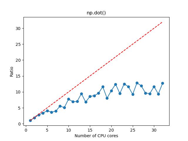
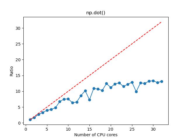
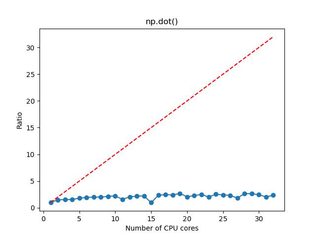
• 对于矩阵乘法，如果矩阵维度较大，那么选择 1~16 核，计算加速的效果比较明显，这时候资源的利用率和性价比也相对比较高；如果矩阵维度较小，那么选择 1~2 核。
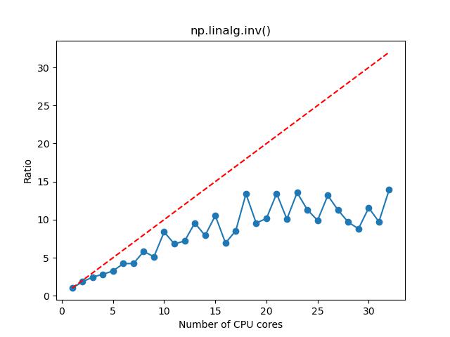
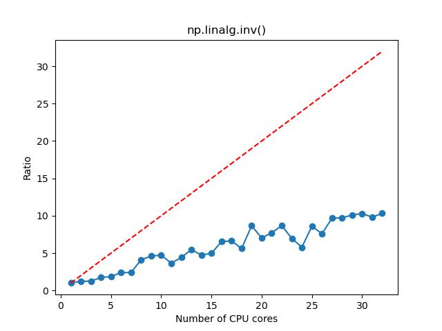
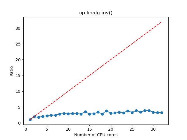
• 对于矩阵求逆，如果矩阵维度较大，那么选择 1~8 核，计算加速的效果比较明显，这时候资源的利用率和性价比也相对比较高；如果矩阵维度较小，那么选择 1~2 核。
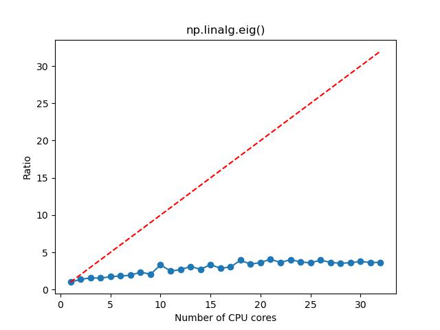
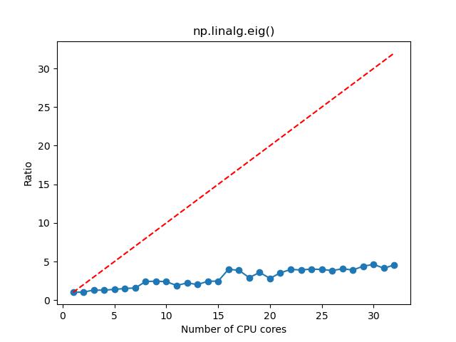
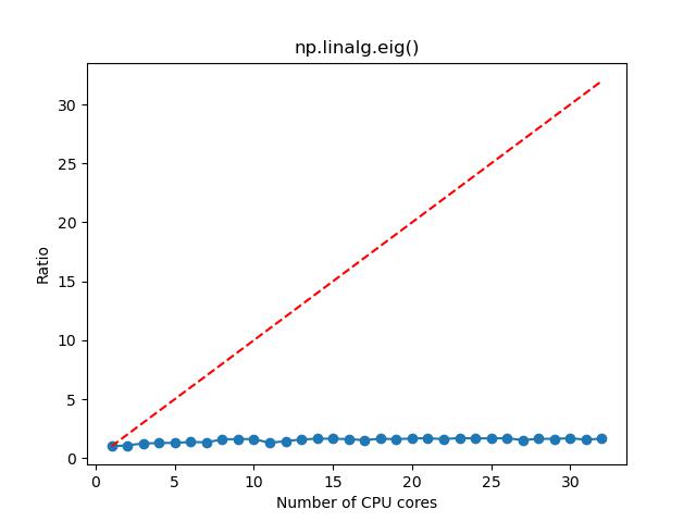
• 对于求解矩阵特征值和特征向量，如果矩阵维度较大，那么选择 1~4 核，计算加速的效果比较明显，这时候资源的利用率和性价比也相对比较高；如果矩阵维度较小，那么选择 1~2 核。

策略选择：

• 在实际的程序中，除了矩阵运算，还有其他一些串行的代码，加速效果不一定那么理想，另外，如果是极小的矩阵，这时候多核也基本上起不到太多的加速作用，因此在以机时为计算成本的情况下，且不追求计算速度，那么使用单核计算的性价比最高。
• 如果希望以尽快速度完成计算，且不占用过多资源，那么推荐以上的核数选择方案。
• 如果资源比较充足，希望以尽快速度完成计算，且不追求资源占用的性价比，那么应该尽量选择最多核数，这样计算速度最快，虽然速度的提升可能会趋于饱和。对于可以大量并行的情况，速度的提升效果会更加明显。

一、测试结果

说明：以下结果为 20 个样本的平均计算时间；n 为矩阵的维度；Ratio 为多核计算时间和单核计算时间相比加速的倍数，具体计算方法见后面的数据处理代码。这里的数据仅为在 P 设备上的测试结果；不同设备由于 CPU 和内存的性能不一样，结果可能会有差别。

1. 矩阵乘积：

2. 矩阵求逆：

3. 矩阵特征值和特征向量：

二、测试代码（手动记录时间，并统计画图）

说明：这部分内容需要手动记录时间，会麻烦了些，可以用于简单测试，对大范围的测试不推荐。

1. 批量生产 PBS 文件的 Python 代码（make_qsub_files.py）：

import guan  # https://py.guanjihuan.com | install: pip install --upgrade guan
import numpy as np

cpu_num_array = np.arange(1, 9)

sh_filename = 'task'
task_name = 'test'
py_filename='matrix_running_time_for_different_num_of_cpu_cores'

for cpu_num in cpu_num_array:
    guan.make_sh_file_for_qsub(sh_filename=sh_filename+'_'+str(cpu_num), command_line=f'python {py_filename}.py', cpu_num=cpu_num, task_name=task_name+'_'+str(cpu_num), cd_dir=0)

2. 提交任务的 PBS 文件示例（task_2.sh，核数为 2）：

#!/bin/sh
#PBS -N test_2
#PBS -l nodes=1:ppn=2
python matrix_running_time_for_different_num_of_cpu_cores.py

3. 批量提交任务 Python 代码（qsub_task.py）：

import numpy as np
import os

cpu_num_array = np.arange(1, 9)

for cpu_num in cpu_num_array:
    os.system(f'qsub task_{cpu_num}.sh')

4. 矩阵运行测试的代码（matrix_running_time_for_different_num_of_cpu_cores.py）：

"""
This code is supported by the website: https://www.guanjihuan.com
The newest version of this code is on the web page: https://www.guanjihuan.com/archives/45324
"""

import numpy as np
import time

n = 1000
test_times = 20

# 矩阵乘法
start_time = time.time()
for _ in range(test_times):
    A = np.random.rand(n, n)
    B = np.random.rand(n, n)
    C = np.dot(A, B)
multiply_time = (time.time() - start_time)/test_times
print(f"矩阵乘法时间: {multiply_time:.3f} 秒")

# 矩阵求逆
start_time = time.time()
for _ in range(test_times):
    A = np.random.rand(n, n)
    inv_A = np.linalg.inv(A)
inv_time = (time.time() - start_time)/test_times
print(f"矩阵求逆时间: {inv_time:.3f} 秒")

# 矩阵的特征值和特征向量
start_time = time.time()
for _ in range(test_times):
    A = np.random.rand(n, n)
    eigenvalues_A, eigenvector_A = np.linalg.eig(A)
eigen_time = (time.time() - start_time)/test_times
print(f"矩阵特征值和特征向量时间: {eigen_time:.3f} 秒")

三、测试代码（时间数据写入文件，使用代码完成统计和画图）【推荐】

1. 批量生产 PBS 文件的 Python 代码（make_qsub_files.py）：

import guan  # https://py.guanjihuan.com | install: pip install --upgrade guan
import numpy as np
import os

cpu_num_array = np.arange(1, 33)

py_filename='matrix_running_time_for_different_num_of_cpu_cores_writing_into_files'
current_directory = os.getcwd()

for cpu_num in cpu_num_array:
    guan.make_directory(f'./task_{cpu_num}')
    os.system(f'cp ./{py_filename}.py ./task_{cpu_num}/{py_filename}.py')
    os.system(f'cd {current_directory}/task_{cpu_num}')
    guan.make_sh_file_for_qsub(sh_filename=f'./task_{cpu_num}/task_{cpu_num}', command_line=f'python {py_filename}.py', cpu_num=cpu_num, task_name=f'test_{cpu_num}', cd_dir=0)

2. 批量提交任务 Python 代码（qsub_task.py）：

import numpy as np
import os

cpu_num_array = np.arange(1, 33)

current_directory = os.getcwd()

for cpu_num in cpu_num_array:
    os.system(f'cd {current_directory}/task_{cpu_num} && qsub {current_directory}/task_{cpu_num}/task_{cpu_num}.sh')

3. 矩阵运行测试的代码（matrix_running_time_for_different_num_of_cpu_cores_writing_into_files.py）：

"""
This code is supported by the website: https://www.guanjihuan.com
The newest version of this code is on the web page: https://www.guanjihuan.com/archives/45324
"""

import numpy as np
import time
import pickle

n = 1000
test_times = 20

# 矩阵乘法
start_time = time.time()
for _ in range(test_times):
    A = np.random.rand(n, n)
    B = np.random.rand(n, n)
    C = np.dot(A, B)
multiply_time = (time.time() - start_time)/test_times
with open(f'multiply_time_n={n}.pkl', 'wb') as f:
    pickle.dump(multiply_time, f)

# 矩阵求逆
start_time = time.time()
for _ in range(test_times):
    A = np.random.rand(n, n)
    inv_A = np.linalg.inv(A)
inv_time = (time.time() - start_time)/test_times
with open(f'inv_time_n={n}.pkl', 'wb') as f:
    pickle.dump(inv_time, f)

# 矩阵的特征值和特征向量
start_time = time.time()
for _ in range(test_times):
    A = np.random.rand(n, n)
    eigenvalues_A, eigenvector_A = np.linalg.eig(A)
eigen_time = (time.time() - start_time)/test_times
with open(f'eigen_time_n={n}.pkl', 'wb') as f:
    pickle.dump(eigen_time, f)

4. 获取数据并画图的 Python 代码（plot_result_of_running_time_by_reading_files.py）：

import matplotlib.pyplot as plt
# from matplotlib.ticker import MultipleLocator
import numpy as np
import pickle

cpu_num_array = np.arange(1, 33)

n = 1000

time_array_1 = []
for cpu_num in cpu_num_array:
    with open(f'./task_{cpu_num}/multiply_time_n={n}.pkl', 'rb') as f:
        data = pickle.load(f)
        time_array_1.append(data)
fig, ax = plt.subplots()
ax.set_title('np.dot()')
ax.set_xlabel('Number of CPU cores')
ax.set_ylabel('Time (s)')
# ax.xaxis.set_major_locator(MultipleLocator(1))
plt.plot(cpu_num_array, time_array_1, '-o', )
plt.savefig(f'multiply_time_n={n}.jpg')
# plt.show()

time_0 = time_array_1[0]
for i0 in range(len(time_array_1)):
    time_array_1[i0] = time_0/time_array_1[i0]
fig, ax = plt.subplots()
ax.set_title('np.dot()')
ax.set_xlabel('Number of CPU cores')
ax.set_ylabel('Ratio')
# ax.xaxis.set_major_locator(MultipleLocator(1))
plt.plot(cpu_num_array, time_array_1, '-o', )
plt.plot(cpu_num_array, cpu_num_array, '--r')
plt.savefig(f'multiply_time_ratio_n={n}.jpg')
# plt.show()


time_array_2 = []
for cpu_num in cpu_num_array:
    with open(f'./task_{cpu_num}/inv_time_n={n}.pkl', 'rb') as f:
        data = pickle.load(f)
        time_array_2.append(data)
fig, ax = plt.subplots()
ax.set_title('np.linalg.inv()')
ax.set_xlabel('Number of CPU cores')
ax.set_ylabel('Time (s)')
# ax.xaxis.set_major_locator(MultipleLocator(1))
plt.plot(cpu_num_array, time_array_2, '-o', )
plt.savefig(f'inv_time_n={n}.jpg')
# plt.show()

time_0 = time_array_2[0]
for i0 in range(len(time_array_2)):
    time_array_2[i0] = time_0/time_array_2[i0]
fig, ax = plt.subplots()
ax.set_title('np.linalg.inv()')
ax.set_xlabel('Number of CPU cores')
ax.set_ylabel('Ratio')
# ax.xaxis.set_major_locator(MultipleLocator(1))
plt.plot(cpu_num_array, time_array_2, '-o', )
plt.plot(cpu_num_array, cpu_num_array, '--r')
plt.savefig(f'inv_time_ratio_n={n}.jpg')
# plt.show()


time_array_3 = []
for cpu_num in cpu_num_array:
    with open(f'./task_{cpu_num}/eigen_time_n={n}.pkl', 'rb') as f:
        data = pickle.load(f)
        time_array_3.append(data)
fig, ax = plt.subplots()
ax.set_title('np.linalg.eig()')
ax.set_xlabel('Number of CPU cores')
ax.set_ylabel('Time (s)')
# ax.xaxis.set_major_locator(MultipleLocator(1))
plt.plot(cpu_num_array, time_array_3, '-o', )
plt.savefig(f'eigen_time_n={n}.jpg')
# plt.show()

time_0 = time_array_3[0]
for i0 in range(len(time_array_3)):
    time_array_3[i0] = time_0/time_array_3[i0]
fig, ax = plt.subplots()
ax.set_title('np.linalg.eig()')
ax.set_xlabel('Number of CPU cores')
ax.set_ylabel('Ratio')
# ax.xaxis.set_major_locator(MultipleLocator(1))
plt.plot(cpu_num_array, time_array_3, '-o', )
plt.plot(cpu_num_array, cpu_num_array, '--r')
plt.savefig(f'eigen_time_ratio_n={n}.jpg')
# plt.show()

5. 提交任务画图（plot_task.sh）：

#!/bin/sh
#PBS -N plot
#PBS -l nodes=1:ppn=1
python plot_result_of_running_time_by_reading_files.py

173 次浏览

【说明：本站主要是个人的一些笔记和代码分享，内容可能会不定期修改。为了使全网显示的始终是最新版本，这里的文章未经同意请勿转载。引用请注明出处：https://www.guanjihuan.com】